Quick Demo: Automatic Data Processing with Solar Data Tools#
8/13/24
This notebook demonstrates the newly added support for the CLARABEL. The SDT pipeline uses CLARABEL by default for all signal decompositions.
Notebook setup and library imports#
[1]:
import numpy as np

# Plotting
import seaborn as sns

sns.set_theme()
sns.set(font_scale=0.8)

# SDT Imports
from solardatatools import DataHandler
from solardatatools.dataio import get_pvdaq_data
Load data from external source#
For today’s example, we’re loading data from NREL’s PVDAQ API, which is a publically available PV generatation data set.
[2]:
data_frame = get_pvdaq_data(sysid=34, year=range(2011, 2015), api_key="DEMO_KEY")
[============================================================] 100.0% ...queries complete in 4.0 seconds
[3]:
data_frame.head()
[3]:
| SiteID | ac_current | ac_power | ac_voltage | ambient_temp | dc_current | dc_power | dc_voltage | inverter_error_code | inverter_temp | module_temp | poa_irradiance | power_factor | relative_humidity | wind_direction | wind_speed | |
|---|---|---|---|---|---|---|---|---|---|---|---|---|---|---|---|---|
| 2011-01-01 00:00:00 | 34.0 | 0.0 | -200.0 | 284.0 | -3.353332 | 0.0 | -200.0 | 16.0 | 0.0 | 37.0 | -7.105555 | 0.0 | 0.0 | 53.513 | 315.270 | 0.483250 |
| 2011-01-01 00:15:00 | 34.0 | 0.0 | -300.0 | 284.0 | -3.381110 | 0.0 | -200.0 | 16.0 | 0.0 | 36.0 | -6.944444 | 0.0 | 0.0 | 53.581 | 308.835 | 0.698724 |
| 2011-01-01 00:30:00 | 34.0 | 0.0 | -300.0 | 284.0 | -3.257777 | 0.0 | -200.0 | 16.0 | 0.0 | 36.0 | -6.344444 | 0.0 | 0.0 | 53.413 | 272.678 | 0.218156 |
| 2011-01-01 00:45:00 | 34.0 | 0.0 | -200.0 | 283.0 | -3.296666 | 0.0 | 0.0 | 15.0 | 0.0 | 36.0 | -6.655555 | 0.0 | 0.0 | 52.406 | 55.913 | 0.159146 |
| 2011-01-01 01:00:00 | 34.0 | 0.0 | -300.0 | 284.0 | -3.426110 | 0.0 | -200.0 | 14.0 | 0.0 | 35.0 | -7.405555 | 0.0 | 0.0 | 53.588 | 152.145 | 0.240508 |
Running the DataHandler processing pipeline#
The Data Handler object takes a DataFrame containing the power data as an input. The DataHandler.run_pipeline method is the main data processing and analysis pipeline offered by Solar Data Tools. It includes preprocessing, cleaning (e.g. fixing time shifts), and scoring data quality metrics (e.g. finding clear days, capacity changes and any clipping).
[4]:
dh = DataHandler(data_frame)
The solver is set the CLARABEL by default. If you’d like to use another solver such as MOSEK, you pass the function the keyword argument solver="MOSEK".
[5]:
dh.run_pipeline(power_col="ac_power")
            *********************************************
            * Solar Data Tools Data Onboarding Pipeline *
            *********************************************

            This pipeline runs a series of preprocessing, cleaning, and quality
            control tasks on stand-alone PV power or irradiance time series data.
            After the pipeline is run, the data may be plotted, filtered, or
            further analyzed.

            Authors: Bennet Meyers and Sara Miskovich, SLAC

            (Tip: if you have a mosek [https://www.mosek.com/] license and have it
            installed on your system, try setting solver='MOSEK' for a speedup)

            This material is based upon work supported by the U.S. Department
            of Energy's Office of Energy Efficiency and Renewable Energy (EERE)
            under the Solar Energy Technologies Office Award Number 38529.
task list: 100%|██████████████████████████████████| 7/7 [00:52<00:00, 7.50s/it]
total time: 52.55 seconds
--------------------------------
Breakdown
--------------------------------
Preprocessing              5.64s
Cleaning                   0.31s
Filtering/Summarizing      46.59s
    Data quality           0.23s
    Clear day detect       0.36s
    Clipping detect        15.64s
    Capacity change detect 30.37s
Top-level reporting#
First we view a quick summary of the data set.
[6]:
dh.report()
-----------------
DATA SET REPORT
-----------------
length               4.00 years
capacity estimate    107.10 kW
data sampling        15 minutes
quality score        0.96
clearness score      0.55
inverter clipping    False
clipped fraction     0.00
capacity changes     False
data quality warning True
time shift errors    False
time zone errors     False
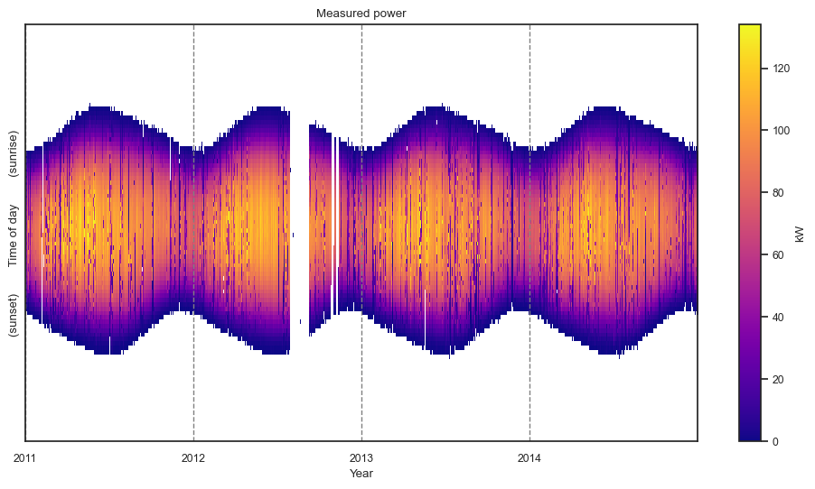
We use heat maps to view the entire data set at once. This provides a much clearer picture of system performance and data set quality than trying to view the time series signal over multiple years.
The “raw” matrix is the initial embedding of the data table after infering the correct shape (number of data points per day by the number of full days) and standardizing the time axis. The white spaces are missing data.
[7]:
dh.plot_heatmap(matrix="raw");
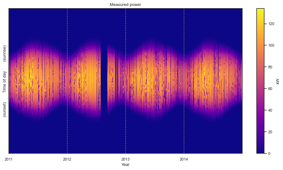
The “filled” matrix is a formal matrix \(M\in\mathbf{R}^{m\times n}\). All entries are real-valued. Night time values and missing days are filled with zeros. Gap within days are filled with linear interpolation.
[8]:
dh.plot_heatmap(matrix="filled", scale_to_kw=True);
Access to data#
Data is available in a number of formats. The first is the original tabular data used at class instantiation.
[9]:
type(dh.data_frame)
[9]:
pandas.core.frame.DataFrame
[10]:
dh.data_frame.columns
[10]:
Index(['SiteID', 'ac_current', 'ac_power', 'ac_voltage', 'ambient_temp',
       'dc_current', 'dc_power', 'dc_voltage', 'inverter_error_code',
       'inverter_temp', 'module_temp', 'poa_irradiance', 'power_factor',
       'relative_humidity', 'wind_direction', 'wind_speed', 'seq_index'],
      dtype='object')
[11]:
dh.data_frame["ac_power"].max()
[11]:
134000.0
[12]:
dh.data_frame["ac_power"].min()
[12]:
-1300.0
The second is the “raw” data matrix. This is a 2D numpy.array object created from the tabular data. Some entries may be missing if there was not a measurement reported for that timestamp in the data table.
[13]:
dh.raw_data_matrix.shape
[13]:
(96, 1461)
[14]:
np.max(dh.raw_data_matrix)
[14]:
nan
[15]:
np.min(dh.raw_data_matrix)
[15]:
nan
Finally, we have the “filled” data matrix. This 2D numpy.array has a real float value in every entry.
[16]:
dh.filled_data_matrix.shape
[16]:
(96, 1461)
[17]:
np.max(dh.filled_data_matrix)
[17]:
134000.0
[18]:
np.min(dh.filled_data_matrix)
[18]:
0.0
Daywise filtering and selection#
After running the pipeline, the class has an attribute which holds a number of boolian indices, each of a length equal to the number of days in the data set. The available flags to filter on are shown below.
[19]:
dh.daily_flags.__dict__.keys()
[19]:
dict_keys(['density', 'linearity', 'no_errors', 'clear', 'cloudy', 'inverter_clipped', 'capacity_cluster'])
[20]:
dh.daily_flags.no_errors
[20]:
array([ True, True, True, ..., True, True, True])
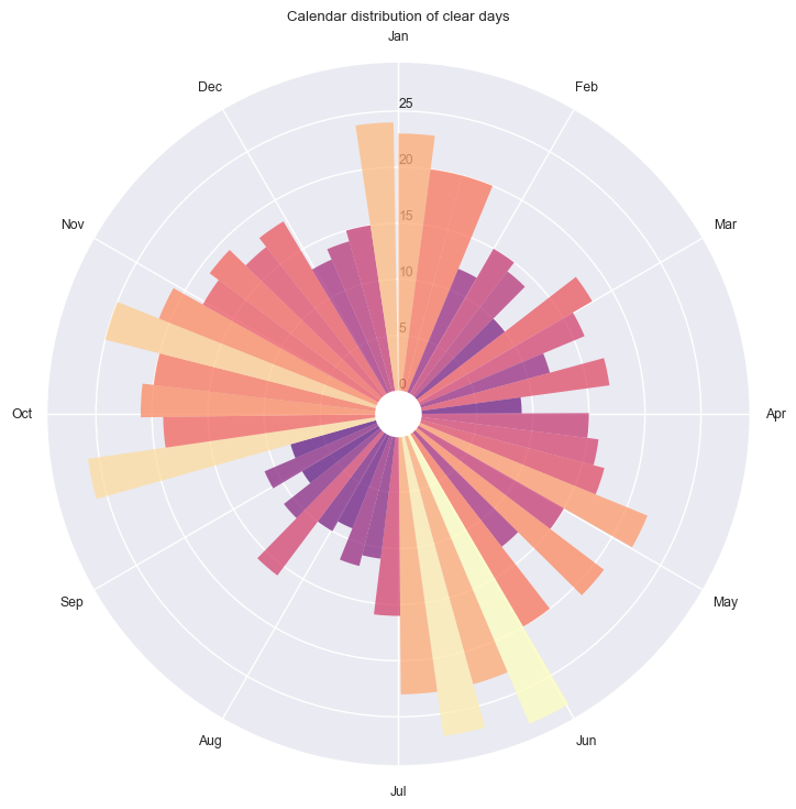
Seasonal analysis using circular statistics#
[21]:
dh.plot_circ_dist(flag="clear");
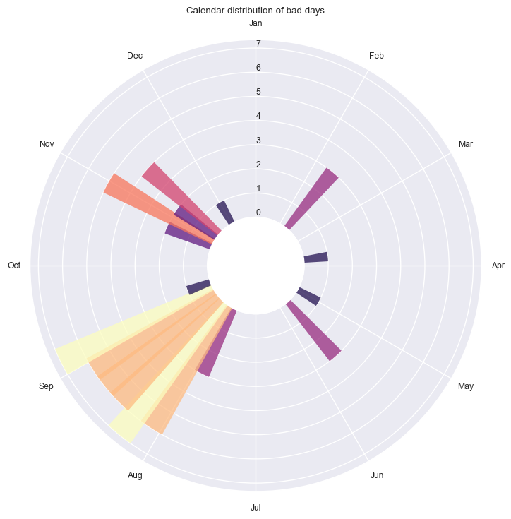
[22]:
dh.plot_circ_dist(flag="bad");
Views into the behavior of the algorithms#
Data quality flagging
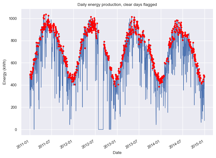
Clear Days#
[23]:
dh.plot_daily_energy(flag="clear");
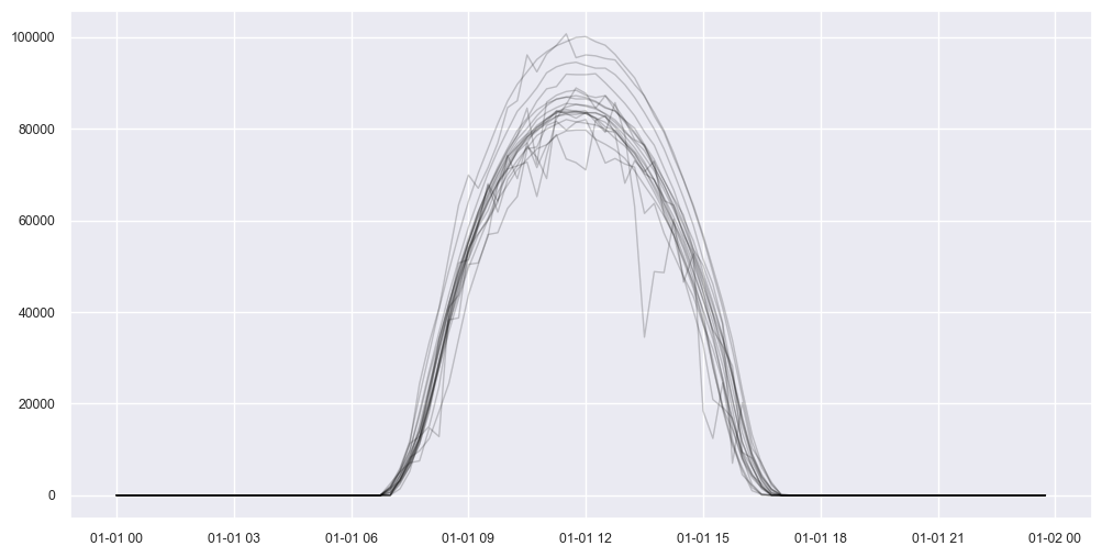
[24]:
bix = dh.daily_flags.clear
dh.plot_daily_signals(
    boolean_index=bix, start_day=0, num_days=20, ravel=False, color="black", alpha=0.2
);
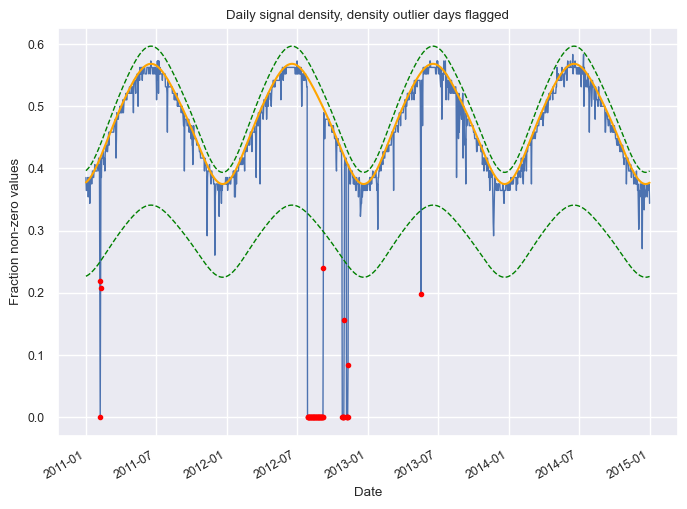
Missing/corrupted data#
[25]:
dh.plot_density_signal(show_fit=True, flag="density");
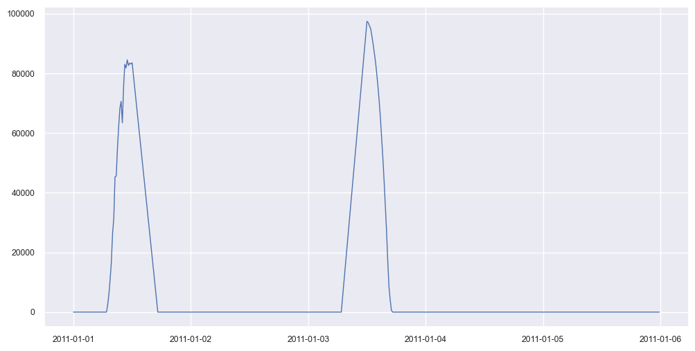
[26]:
# Select days that failed the density test
bix = ~dh.daily_flags.density
dh.plot_daily_signals(boolean_index=bix, start_day=0, num_days=5, ravel=True);
[27]:
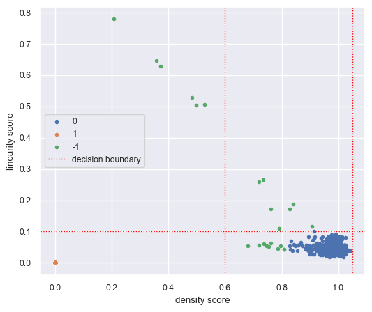
dh.plot_data_quality_scatter();
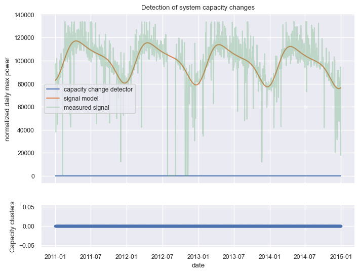
Capacity change analysis#
This analysis checks for abrupt step changes in the apparent capacity of the system.
[28]:
dh.plot_capacity_change_analysis();
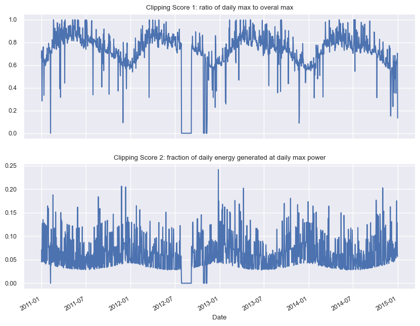
Clipping analysis#
These plots show how clipped days are detected (none in this data set).
[29]:
dh.plot_clipping();
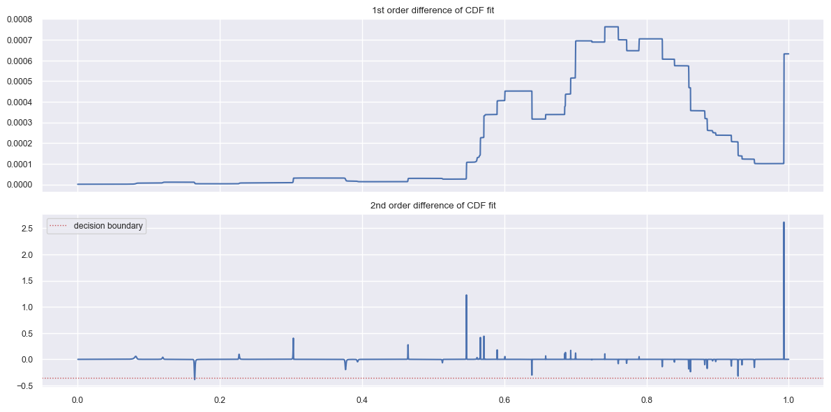
[30]:
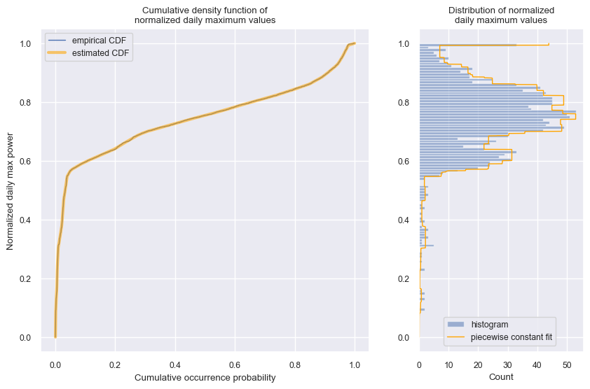
dh.plot_cdf_analysis();
[31]:
dh.plot_daily_max_cdf_and_pdf();
Timeshift analysis#
These plots show the results of the time shift analysis algorithm that corrects any detected shifts in the data.
[32]:
# This should not plot anything as we have not fixed any shifts in the pipeline run
dh.plot_time_shift_analysis_results()
Please run pipeline first.
We should run the pipeline with fix_shifts=True first to invoke the time shift analysis algorithm:
[33]:
dh.run_pipeline(power_col="ac_power", fix_shifts=True)
            *********************************************
            * Solar Data Tools Data Onboarding Pipeline *
            *********************************************

            This pipeline runs a series of preprocessing, cleaning, and quality
            control tasks on stand-alone PV power or irradiance time series data.
            After the pipeline is run, the data may be plotted, filtered, or
            further analyzed.

            Authors: Bennet Meyers and Sara Miskovich, SLAC

            (Tip: if you have a mosek [https://www.mosek.com/] license and have it
            installed on your system, try setting solver='MOSEK' for a speedup)

            This material is based upon work supported by the U.S. Department
            of Energy's Office of Energy Efficiency and Renewable Energy (EERE)
            under the Solar Energy Technologies Office Award Number 38529.
task list: 100%|██████████████████████████████████| 7/7 [00:48<00:00, 6.89s/it]
total time: 48.24 seconds
--------------------------------
Breakdown
--------------------------------
Preprocessing              4.75s
Cleaning                   3.44s
Filtering/Summarizing      40.06s
    Data quality           0.20s
    Clear day detect       0.34s
    Clipping detect        11.00s
    Capacity change detect 28.52s
Then we can try plotting the results again.
[35]:
dh.plot_time_shift_analysis_results();
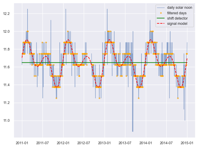
As you can see with the flat green “shift detector line”, no time shifts were detected (as we expected by looking at the heatmap plotted above).
[ ]: