Demonstration of statistical clear sky fitting#
6/24/2025
This notebook demontrates how to use the newly updated clear sky fitting method, based on smooth, periodic quantile estimation. The basic steps are:
load data
run pipeline
estimate clear sky model
Notebook setup and library imports#
[1]:
from solardatatools import DataHandler, plot_2d
from solardatatools.dataio import get_pvdaq_data
Load data#
We use NREL’s PVDAQ API with a function from the Solar Data Tools DataIO module
[2]:
data_frame = get_pvdaq_data(sysid=34, year=range(2011, 2015), api_key="DEMO_KEY")
[============================================================] 100.0% ...queries complete in 3.2 seconds
Run main pipeline#
[3]:
dh = DataHandler(data_frame)
dh.run_pipeline(power_col="ac_power")
            *********************************************
            * Solar Data Tools Data Onboarding Pipeline *
            *********************************************

            This pipeline runs a series of preprocessing, cleaning, and quality
            control tasks on stand-alone PV power or irradiance time series data.
            After the pipeline is run, the data may be plotted, filtered, or
            further analyzed.

            Authors: Bennet Meyers and Sara Miskovich, SLAC

            (Tip: if you have a mosek [https://www.mosek.com/] license and have it
            installed on your system, try setting solver='MOSEK' for a speedup)

            This material is based upon work supported by the U.S. Department
            of Energy's Office of Energy Efficiency and Renewable Energy (EERE)
            under the Solar Energy Technologies Office Award Number 38529.
task list: 100%|██████████████████████████████████| 7/7 [00:09<00:00, 1.38s/it]
total time: 9.67 seconds
--------------------------------
Breakdown
--------------------------------
Preprocessing              2.18s
Cleaning                   0.11s
Filtering/Summarizing      7.38s
    Data quality           0.08s
    Clear day detect       0.16s
    Clipping detect        3.24s
    Capacity change detect 3.89s
Fit clear sky model#
The nvals_dil parameter controlls how many data points used each day in the model. The higher the number of values, the longer the fit time (and it scales linearly).
5-minute data has 288 data points per day, roughly 50% of which are nighttime zeros, on average, and so the default is set to nvals_dil=101, to give you 100 data points between sunrise and sunset plus one “nighttime” value.
This data example happens to have 15-minute data, or 96 data points per data. Setting nvals_dil=31 avoids excessive upsampling of the data and reduces the fit time for the clear sky model by 1/3.
the regularization parameter controls the “stiffness” of the fit, with high values resulting in less “wiggly” fits. The defualt value is 0.1, and we bumped it up to 1.0 for this example (simple data set with not a lot of variability or shade effects).
[16]:
dh.fit_statistical_clear_sky_model(nvals_dil=31, regularization=1)
100%|█████████████████████████████████████████████| 1/1 [01:06<00:00, 66.79s/it]
[17]:
dh.plot_daily_signals(show_clear_model=True, start_day=650);
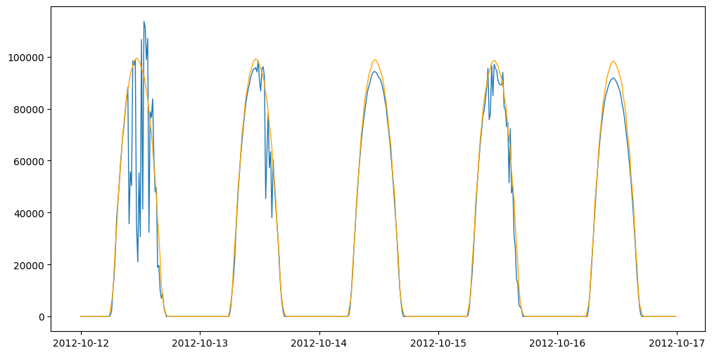
The estimated clear sky signal is available in the self.scsf attribute
[18]:
dh.scsf
[18]:
array([808.74757358, 808.74757358, 808.74757358, ...,   0.        ,
         0.        ,   0.        ], shape=(140256,))
The clear sky fitting module is a wrapper on the more general quantile estimation module. As seen below, estimating the clear sky model is the same as estimating the 0.9 quanile.
[19]:
dh.quantile_object.quantiles_original
[19]:
{np.float64(0.9): array([808.74757358, 808.74757358, 808.74757358, ...,   0.        ,
          0.        ,   0.        ], shape=(140256,))}
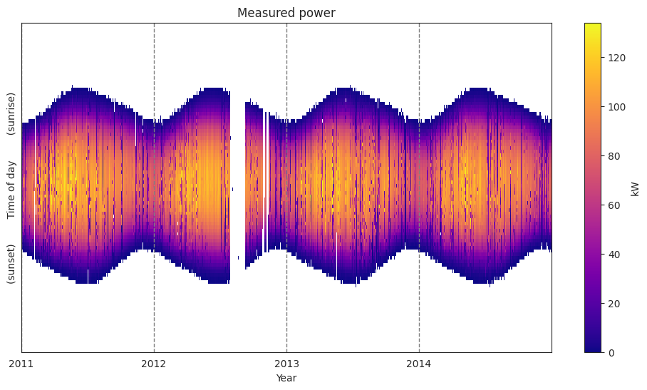
Compare actual and estimated power heatmaps#
measured power:
[20]:
dh.plot_heatmap('raw');
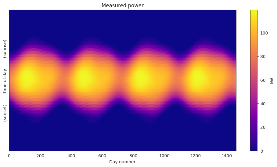
estimated clear sky system response:
[21]:
plot_2d(dh.scsf.reshape(dh.raw_data_matrix.shape, order='F')/1000);